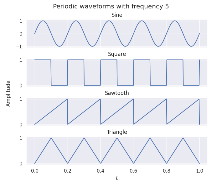
Matplotlib, decorators and plotting waves

In this tutorial, we will learn how generatate plots using Matplotlib and Numpy. Specifically we'll plot waveforms, which in our context just means periodic functions (i.e. functions $f$ such that $f(x + P) = f(x)$ for some $P$

Let's start by defining some key terms of waveforms: the period of a wave is the time it takes for one complete oscillation to occur; the frequency of a wave is the number of oscillations that occur in a given period of time and the amplitude of a wave is the measure of the height of the wave, it is the distance between the crest or trough and the mean position of the wave.

Once we have a basic understanding of these concepts, we can move on to using Matplotlib to plot waveforms. We will begin by plotting a single period wave, and then use a function decorator to make it periodic.

There are many different types of waveforms, each with its own unique characteristics and applications. In this tutorial we will be plotting four of the most commonly seen shapes: Square, Triangular, Sawtooth and Sine

Setting up our project

Those are de dependencies we will be using for this project:

matplotlib
scipy
numpy
seaborn

Install them to your virtual env, then create a python file and import the libs and methods we will be using in our project

touch plotting.py

import matplotlib.pyplot as plt
import seaborn as sns
import numpy as np

Now let's have some fun plotting waveforms:

Defining functions

The first thing we wanna do is define each one of the functions we will be using to plot our waveforms:

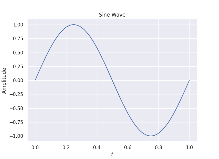
Sine Wave: The function $B_p: [0, 1]\longrightarrow [0, 1]$ that describes a single period of a sine wave is given by:

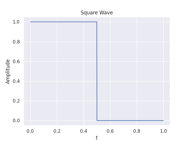
$\begin{equation} B_p(x)= \sin(2\pi x) \end{equation}$

Square Wave: The function $S_p: [0, 1]\longrightarrow [0, 1]$ that describes a single period of a square wave is given by:

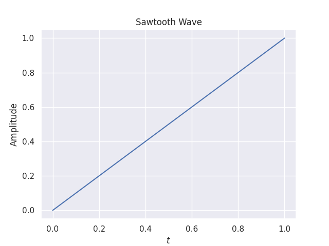
$\begin{equation} S_p(x)= \begin{cases} 1, \quad \text{if } x < 0.5 \\ 0, \quad \text{if } x > 0.5 \end{cases} \end{equation}$

Sawtooth Wave: The function $W_p: [0, 1]\longrightarrow [0, 1]$ describes one period of a sawtooth wave. It is defined as:

$\begin{equation} W_p(x)= x \end{equation}$

Triangle Wave: The function $T_p: [0, 1]\longrightarrow [0, 1]$ represents one cycle of a triangle wave and is defined as:

$\begin{align} T_p(x)= \begin{cases} 2x, &\text{if } x < 0.5 \\ -2x + 2, &\text{if } x > 0.5 \end{cases} \end{align}$

Translating our mathematical functions into python code

Now Let's translate each one of the functions above into code. For that, we will be using numpy piecewise method that, uppon receiving a set of conditions and corresponding functions, evaluate each function on the input data wherever its condition is true.

def sine_wave(X):
    Y = np.sin(2 * np.pi * X)
    return Y

def square_wave(X):
  Y = np.piecewise(X, [X < 0.5, X >= 0.5], [1, 0])
  return Y

def sawtooth_wave(X):
    Y = X
    return Y

def triangle_wave(X):
    Y = np.piecewise(X, [X < 0.5, X >= 0.5], [lambda X: X * 2, lambda X: -X * 2 + 2])
    return Y

To define the X values we will be passing to our functions, we will now use another numpy method called linspace that return evenly spaced numbers over a specified interval (in our case from 0 to 1)

X = np.linspace(0, 1, 500)

Plotting single period waveforms

Now that we have our variables set up, we can plot each waveform using matplotlib.plyplot.plot() function.

This function, by default, receives two parameters (1 being an array containing the points on the x-axis and 2 being an array containing the points on the y-axis) and draws a line from point to point in a diagram.

As you might have noticed, the number of points, in our case, is defined by the ammount of numbers returned by the np.linspace method we used before.

To make our plots more readable we will add a title and labels for our x and y-axis:

def sine_wave(X):
  Y = np.sin(2 * np.pi * X)
  return Y

X = np.linspace(0, 1, 500)
Y = sine_wave(X)

plt.title("Sine Wave")
plt.xlabel(r"$t$")
plt.ylabel(r"Amplitude")
plt.plot(X, Y)

plt.show()

An image of a single period sine wave

def square_wave(X):
  Y = np.piecewise(X, [X < 0.5, X >= 0.5], [1, 0])
  return Y

X = np.linspace(0, 1, 500)
Y = square_wave(X)

plt.title("Square Wave")
plt.xlabel(r"$t$")
plt.ylabel(r"Amplitude")
plt.plot(X, Y)

plt.show()

An image of a single period square wave

def sawtooth_wave(X):
    Y = X
    return Y

X = np.linspace(0, 1, 500)
Y = sawtooth_wave(X)

plt.title("Sawtooth Wave")
plt.xlabel(r"$t$")
plt.ylabel(r"Amplitude")
plt.plot(X, Y)

plt.show()

An image of a single period sawtooth wave

def triangle_wave(X):
  Y = np.piecewise(X, [X < 0.5, X >= 0.5], [lambda X: X*2, lambda X: -X*2 + 2])
  return Y

X = np.linspace(0, 1, 500)
Y = triangle_wave(X)

plt.title("Triangle Wave")
plt.xlabel(r"$t$")
plt.ylabel(r"Amplitude")
plt.plot(X, Y)

plt.show()

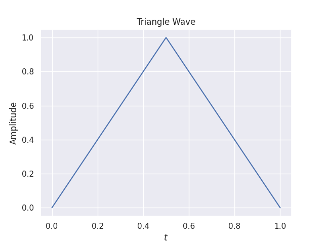
An image of a single period triangle wave

Once we have our single period functions defined and plotted, it's now time to make them periodic, to do that we will be using function decorators:

Decorators

What are decorators? Decorators are functions that takes another function as argument and modify its behavior without explicity changing it. This definition might be a little cryptic so let's build an example to ilustrate it

We will start by defining a very simple function that takes no argument and prints a string:

def my_func():
    print "function to be decorated"

the output for this function is:

$ my_func()

#"function to be decorated"

Then we will create a function my_decorator that takes another function as argument and simply prints a string before the argument function is called:

def my_func():
    print "function to be decorated"

def my_decorator(func):
    def wrapper():
        print "this function is now decorated"
        func()
    return wrapper

After that we will assign the decorator function to the main function, passing the main function as the argument:

def my_func():
    print "function to be decorated"

def my_decorator(func):
    def wrapper():
        print "this function is now decorated"
        func()
    return wrapper

my_func = my_decorator(my_func)

When called, the output for my_func should be:

$ my_func()

#"this function is now decorated"
#"function to be decorated"

As you can see the decorator changed the functionality of the function by wrapping it in another function.

You might have noticed that the way we decorated our function is a little clunky, verbose, and it kind of hides the decoration below the definition of the function. Thankfuly Python provides a more elegant way of declaring decorators using the @ symbol.

def my_decorator(func)
    def wrapper():
        print "this function is now decorated"
        func()
    return wrapper

@my_decorator
def my_func():
    print "function to be decorated"

The code above does exactly the same thing we did when we declared my_func = my_decorator(my_func).

Now that you have a basic understandig of what decorators do and how to use them, we can make it a little more interesting:

Suppose we want to create a function, decorate it in a way that any given number is multiplied by 2 and then display the result

First we will define a function that takes an int as argument and simply return its value:

def return_a_number(x):
    return x

It is possible to pass arguments to the decorator itself, but to use its values we need do add another wrapper function that will receive and pass the function the same way the decorator did before. Let's see how it works:

def multiplier_decorator(number):
  def outer_wrapper(function_to_be_multiplied):
    def wrapper(function_to_be_multiplied_argument):
      result = my_func(function_to_be_multiplied_argument * number)
      print(result)
    return wrapper
  return outer_wrapper

Now that our decorator is ready and our function is defined, lets decorate it. In this case, the argument we will be passing to the decorator is the number we want the x value to be multiplicated by, namely 2

def multiplier_decorator(number):
  def outer_wrapper(function_to_be_multiplied):
    def wrapper(function_to_be_multiplied_argument):
      result = my_func(function_to_be_multiplied_argument * number)
      print(result)
    return wrapper
  return outer_wrapper

@multiplier_decorator(2)
def return_a_number(x):
    return x

$ return_a_number(5)

#10

Making our functions periodic

Our next goal is transform the single-period waveforms we defined above ( $Sp$ , $Wp$ and $Tp$ ) into actual periodic functions with some frequency $F$ .

A function $h$ is said to be periodic with period $P$ if and only if $h(x) = h(x + P)$ for all $x$ in its domain. It is of course clear that if a function has period $P$ (i.e. the width along the x-axis - or duration, if we’re thinking of the x-axis as time - of a single period is $P$ ), then it has a frequency $F=\frac{1}{P}$ (i.e. it completes $\frac{1}{P}$ periods per unit of length/time). It turns out that we can achieve the above by using function composition. We define a new function $g$ :

$\begin{align} g: \mathbb{R} &\longrightarrow [0,1] \\ x &\longmapsto (Fx) \bmod 1 \end{align}$

where we’re using the (binary) modulo $operator$ . Notice that the range of this function is $[0, 1]$ - this is ensured by the modulo operator - which is exactly the domain of our single-period functions. We can then construct a periodic function $h$ with frequency $F$ using a single period function $f$ (defined in the $[0, 1]$ interval) as $h = f \circ g$ . Specifically

$\begin{align} h: \mathbb{R} &\longrightarrow [0,1] \\ x &\longmapsto (f \circ g)(x) = f(g(x)) \end{align}$

Intuitively, what’s happening here is that the function $g$ is doing two things. The first is that it’s squashing or stretching (depending on whether $F$ is smaller or greater than $1$ , respectively) the single period - this is accomplished by the $Fx$ term. The second is that it’s creating the repetitions themselves by using the mod operator after the squash/stretch operation.

We can give a very simple proof that the function $h$ , as defined above, is periodic with period $\frac{1}{F}$ for any function $f$ defined in the range $[0, 1]$ . For this, we’ll need two properties of the binary mod operator:

$\begin{align} (a + b) \bmod c &= (a \bmod c + b \bmod c) \\ (a \bmod c) \bmod c &= a \bmod c \end{align}$

We then make use of the definition given above for a periodic function. That is, showing that the resulting function $h = (f \circ g)$ is periodic with period $\frac{1}{F}$ is equivalent to showing that $h(x) = h \left( x + \frac{1}{F} \right)$ for all $x$ in it’s domain (in this case, the domain is the set of real numbers, i.e. $\mathbb{R}$ ). So we take an arbitrary real number x and an arbitrary function f defined in the $[0, 1]$ interval and compute

$\begin{align} h(x) &= (f \circ g)(x) \\ &= f (g(x)) \\ &= f (Fx \bmod 1) \end{align}$

On the other hand:

$\begin{align} h \left( x + \frac{1}{F} \right) &= (f \circ g)(x + \frac{1}{F}) \\ &= f \left( g(x + \frac{1}{F}) \right) \\ &= f \left( F(x + \frac{1}{F}) \bmod 1 \right) \\ &= f ( (Fx +1) \bmod 1 ) \\ &= f ( (Fx \bmod 1 + 1 \bmod 1) \bmod 1 ) \\ &= f ( (Fx \bmod 1) \bmod 1 ) \\ &= f ( Fx \bmod 1 ) \end{align}$

Where the first 4 equalities are just definitions and substitutions, the 5th makes use of property number 1 of the mod operator, and the last equality makes use of property number 2

Comparing the two final expressions above, we see that indeed $h(x) = h \left( x + \frac{1}{F} \right)$ (they’re both equal to $f(Fx \bmod 1))$ , which proves that $h$ is periodic with period $\frac {1}{F}$ .

It is worth mentioning that the reason why we used $g(x) = Fx \bmod 1$ , rather than, say $g(x) = Fx \bmod 72.5$ , is that our original function is defined in the range $[0, 1]$ . If we wanted the single period to be given by a function in the range $[0, a]$ for any positive real number $a$ , then we would need to use $g(x) = (aFx) \bmod a$ and everything would work out exactly the same.

We are now in a position to define $S$ , $W$ and $T$ - the periodic versions of our waveforms:

$\begin{align} S &= Sp \circ h \\ W &= Wp \circ h \\ T &= Tp \circ h \\ \end{align}$

Plotting periodic functions

As we defined above, the function $g(x)$ that describes a repeating pattern associated to a frequency $F$ in an interval $[0,1]$ is given by:

$\begin{equation} g(x)= xF \mod 1 \end{equation}$

wich can be translated to python code as:

def g(X):
    return X * frequency % 1

Now what we want to do is to pass $g(x)$ as an argument to our single period functions - i.e. $f(g(x))$ .

But how can we do that in our code since, in principle, our functions responsability is to describe a single period of a given wave and receives as argument only the values of X corresponding to that single occurance in the interval $[0, 1]$ ?

That's when what we learned about decorators comes in play. In our last example we saw that we can pass an value as argument to our decorator and then use it to change the function we are decorating. In our case, the value we want to pass is the frequency as this is the only missing piece to complete our g(X) function that we want to pass as argument to the single period function.

With that in mind, let's build our decorator:

def make_periodic(frequency):
  def outer_wrapper(single_period_func):
    def wrapper(X):
      result = single_period_func(X * frequency % 1)
      return result
    return wrapper
  return outer_wrapper

We can now decorate our single wave functions to be ploted with any given frequency. Suppose we want to plot them all with a frequency of 5. All we have to do is add our decorator to them passing 5 as the argument of our decorator.

def make_periodic(frequency):
  def outer_wrapper(single_period_func):
    def wrapper(X):
      result = single_period_func(X * frequency % 1)
      return result
    return wrapper
  return outer_wrapper

@make_periodic(5)
def sine_wave(X):
  Y = np.sin(2 * np.pi * X)
  return Y

@make_periodic(5)
def square_wave(X):
  Y = np.piecewise(X, [X < 0.5, X >= 0.5], [1, 0])
  return Y

@make_periodic(5)
def sawtooth_wave(X):
  Y = X
  return Y

@make_periodic(5)
def triangle_wave(X):
  Y = np.piecewise(X, [X < 0.5, X >= 0.5], [lambda X: X*2, lambda X: -X*2 + 2])
  return Y

Finally, let's plot our periodic waves. To stack them in a single plot we will be using matplotlib plt.subplots that allows you to define multiple axis values

def make_periodic(frequency):
  def outer_wrapper(single_period_func):
    def wrapper(X):
      result = single_period_func(X * frequency % 1)
      return result
    return wrapper
  return outer_wrapper

@make_periodic(5)
def sine_wave(X):
  Y = np.sin(2 * np.pi * X)
  return Y

@make_periodic(5)
def square_wave(X):
  Y = np.piecewise(X, [X < 0.5, X >= 0.5], [1, 0])
  return Y

@make_periodic(5)
def sawtooth_wave(X):
  Y = X
  return Y

@make_periodic(5)
def triangle_wave(X):
  Y = np.piecewise(X, [X < 0.5, X >= 0.5], [lambda X: X*2, lambda X: -X*2 + 2])
  return Y

X = np.linspace(0, 1, 500)
Y0 = sine_wave(X)
Y1 = square_wave(X)
Y2 = sawtooth_wave(X)
Y3 = triangle_wave(X)

fig, axs = plt.subplots(4, sharex=True)
plt.xlabel(r"$t$")
fig.text(0.04, 0.5, r"Amplitude", va="center", ha="center", rotation="vertical")
fig.suptitle("Periodic waveforms with frequency 5")
axs[0].plot(X, Y0)
axs[1].plot(X, Y1)
axs[2].plot(X, Y2)
axs[3].plot(X, Y3)
axs[0].title.set_text("Sine")
axs[1].title.set_text("Square")
axs[2].title.set_text("Sawtooth")
axs[3].title.set_text("Triangle")
plt.show()

The resulting plot should resemble this.:

An image of periodic waveforms